Let’s Brush up quickly what we have learnt so far:-
I highly recommend to read the previous blog befor you dive in.
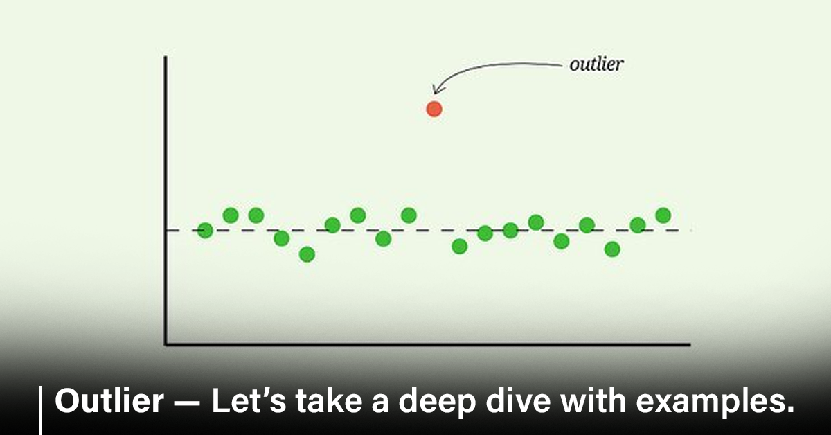
Outlier — An odd & special one out
An outlier can be defined as a data point that deviates significantly from the normal pattern or behavior of the data.

Scenario — 1
Let’s see with an example, the table below shows the number of messages exchanged on the smart phones of 14 students over a single month. The data have also been plotted in a dot plot.
Are there any outliers in this data set? If so, specify the value or values of these outliers.
Answer
If we consider the graph, we can see that one data point at the far right end is a long way from the rest of the data. The value appears to be fairly close to 10 000 and looking in the table we can see that there is one data point with the value 9 754.
Given that the rest of the data appear to have values less than 5 500, we can conclude that 9 754 is an outlier.
Small Exercise
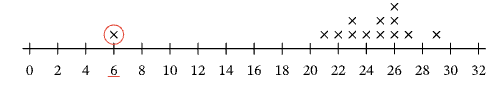
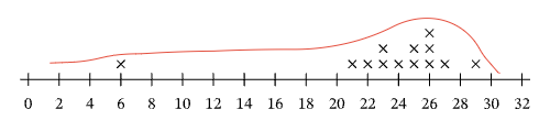
Which of the statements is correct for the distribution represented by the diagram?
- The distribution has an outlier at 6.
- The distribution is symmetric.
- The distribution has a gap from 21 to 29.
- The distribution has a cluster from 7 to 20.
- The distribution has a peak at 22.
Answer
To find which of the statements is correct, we will consider them one by one.
(1) This is the statement: The distribution has an outlier at 6. Looking at the graph, there is a single data point marked with a cross above the value “6.”
The next value on the axis with a cross above it, signifying a data point, is 21; and between the data point at 6 and this one, there are 21−6=15 values.
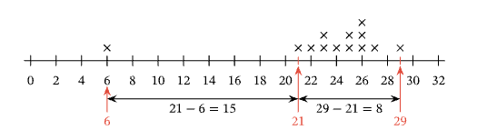
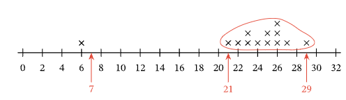
Given that the rest of the data clusters between 21 and 29, we can say that the data point at 6 is quite far removed from the rest of the data. Hence, the distribution does have an outlier at 6 and answer (1) is correct.
(2) This is the statement: The distribution is symmetric. If we trace out the distribution, we can see that, with the outlier at 6, the shape of the distribution is not symmetric.
Answer (2) is then incorrect. In fact, the distribution is stretched by the data point at 6.
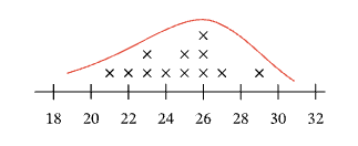
Note that if we were to remove this data point, all of our remaining data would be between 21 and 29.
Tracing the distribution of this new data set, without the point at 6, we can see that it is fairly symmetric, or at least more so than the original data set. It is clear then that the outlier at 6 distorts the distribution of the original data set.
(3) This is the statement: The distribution has a gap from 21 to 29. This is clearly untrue as in fact the majority of the data lie between 21 and 29.
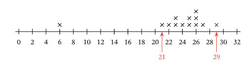
(4) This is the statement: The distribution has a cluster from 7 to 20. This is clearly untrue. There is a cluster of data points, but the cluster is from 21 to 29.
(5) This is the statement: The distribution has a peak at 22. This statement is incorrect. There is a single data point with the value 22 and this does not represent a peak. The value with the most data points above it on the graph is 26, with 3 data points valued at 26.
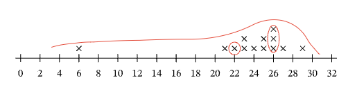
Tracing out the curve of the distribution, we can see that above 26 is the highest point on the curve. We can therefore say that there is a peak at 26, but not at 22.
In conclusion, answer (A) is the only correct answer: The distribution has an outlier at 6.
Scenario — 2
How an Outlier Can Affect a Data Set
The data in the table below is the average recorded speed, in miles per hour, of the first serve of the top 10 tennis players in the world.

- Calculate the mean 1st serve speed in miles per hour.
- Recalculate the mean 1st serve speed without the data point 1 025 mph.
- By comparing the means you found in the first two parts of the question, make a conclusion about the validity of the 1 025 mph data point.
Part 1
To calculate the mean 1st serve speed, we need to add up all the speeds and divide by the number of players whose speeds are in the data set. The sum of all the speeds is
126 + 115 + 99 + 136 + 105 + 138 + 121 + 1025 + 118 + 124 = 2107.
mean speed = sum of speeds / number of Players
2107 / 10 = 210.7 mph
The mean 1st serve speed for the top ten tennis players is therefore 210.7 miles per hour.
Part 2
To recalculate the mean without the value of 1 025 miles per hour,
we have the new sum:-
126 + 115 + 99 + 136 + 105 + 138 + 121 + 118 + 124 = 1082.
We now only have 9 values, so our new mean speed is:-
mean speed = sum of speeds / number of Players
1082/9=120.2 mph
Part 3
With the value 1 025 mph included in our calculation, we found a mean 1st serve speed of 210.7 mph. Apart from the recorded speed of 1 025 miles per hour, this mean is substantially higher than any of the other speeds recorded. Since the mean is a measure of the center of the data, a mean this high does not make sense as it is not close in value to any of the data.

Also, considering the recorded speed of 1 025 mph,it does not seem possible for even one of the top players in the world to have an average first serve speed of 1 025 mph!
We must conclude that this value is an outlier and must in fact be an error.

Calculating the mean without this value, we find the mean 1st serve speed is 120.2 mph, which makes much more sense, since its value is close to the majority of the data.